from pandas import json_normalize
import requests
import plotly.express as px
import plotly.io as pio
pio.renderers.default = "plotly_mimetype+notebook_connected"
import plotly.graph_objects as go
from plotly.subplots import make_subplots
import base64
from IPython.display import Image, display
def mm(graph):
graphbytes = graph.encode("ascii")
base64_bytes = base64.b64encode(graphbytes)
base64_string = base64_bytes.decode("ascii")
display(Image(url="https://mermaid.ink/img/" + base64_string))1 An artist’s analysis
In this first part I’m going to work with the /artist/{id} session of the Spotify API. With this functionality general data can be extracted. This general data contains things as genres, popularity and followers. I will also work with the artist’s top 10 songs to make a very general summary of the artist’s profile, which will give us ideas about their years of popularity, duration of the songs and most well-known albums.
1.1 API
A small summary of the functionalities that I will use:
GET /artist/{id}
GET /artist/{id}/albums
GET /artist/{id}/top-tracks| Parameter | Type | Description |
|---|---|---|
| id (required) | string |
Get Spotify catalog information for a single artist identified by their unique Spotify ID.The ID of the artist. |
| albums | string |
Get Spotify catalog information about an artist’s albums. |
| top-tracks | string |
Get Spotify catalog information about an artist’s top tracks by country. |
As I use each parameter, I will explain the configuration and filtering options they have.
1.2 Libraries
I import the libraries I will need:
1.3 Configuration
Before thinking about making requests to obtain data, you must first create an app in Spotify, this app will give you the possibility to authenticate yourself and make the requests that are needed. To make this app you can go to this link where you will find all the necessary information. Link
After the app has been created, the authentication data is delivered, similar to these:
CLIENT_ID = '81e800e81ecf4997b5b9fb12efeb3ff2'
CLIENT_SECRET = '0e4364f440f148779d8a9f17976ecf1b'
(These were removed after making this publication)
When the app authenticates, Spotify will return a token, this token is the one used in the header to make all requests. All tokens have a time to live, I’m not sure, but I think it’s 3600 seconds, I recommend looking at the documentation if this may be a problem for you.
In the following code blocks I show how to create a function to get this token and then store it in the header variable.
# Function to get the token
def get_token():
    url = 'https://accounts.spotify.com/api/token'
    auth_response = requests.post(url, {
        'grant_type': 'client_credentials',
        'client_id': CLIENT_ID,
        'client_secret': CLIENT_SECRET,
    })
    if auth_response.status_code != 200:
        raise Exception('Error getting token')
    else:
        auth_response_data = auth_response.json()
        return auth_response_data['access_token']
# Get token
access_token = get_token()
header = {
'Authorization': 'Bearer {token}'.format(token=access_token),
'accept':'application/json'
}base_url = 'https://api.spotify.com/v1/'1.4 Workflow
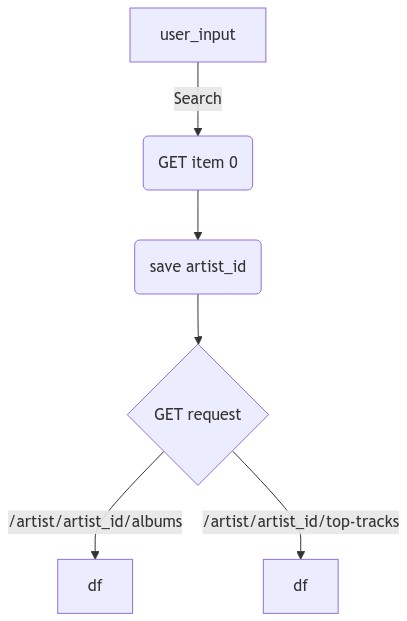
The workflow from when the user enters the name of the artist until it is saved in the dataframes is represented in the following diagram
mm("""
graph TD
    A[user_input] -->|Search| B(GET item 0)
    B --> C(save artist_id )
    C --> D{GET request}
    D -->|/artist/artist_id/albums| E[df]
    D -->|/artist/artist_id/top-tracks| F[df]
""")
1.5 Artist profile
I ask the user to enter the name of the user they want to analyze, and then I use Spotify’s search to get the artist ID.
The ID is a unique text string for each artist/song/album or list and this ID is one of the most important parameters to make requests since it allow us to have more precision in our needs.
The output of the search is a list, and I take the first result.
#ask for user input for artist name
artist_name = input('Enter artist name: ')
print('the artist name is: ', artist_name)
the artist name is: Rush#get artist id
artist_id = requests.get(base_url + 'search?q={}&type=artist'.format(artist_name), headers=header).json()['artists']['items'][0]['id']The structure of the json object delivered by /artist/{id} can be found at this link. Link
#get artist profile
r_artist_profile = requests.get(base_url + 'artists/{}'.format(artist_id), headers=header).json()
df_artist = json_normalize(r_artist_profile)
df_artist.columns
Index(['genres', 'href', 'id', 'images', 'name', 'popularity', 'type', 'uri',
'external_urls.spotify', 'followers.href', 'followers.total'],
dtype='object')I don’t need all this information, so I select only the necessary columns:
df_artist.drop(['images', 'uri', 'href', 'followers.href','type'], axis=1, inplace=True)I always change the name of the columns to make it easier to read and understand the data.
#change column names
df_artist.columns = ['Genres', 'ID', 'Artist', 'Popularity', 'URL', 'Followers']
And finally a have a very brief overview of the artist:
df_artist.transpose()| 0 | |
|---|---|
| Genres | [album rock, art rock, canadian metal, classic... |
| ID | 2Hkut4rAAyrQxRdof7FVJq |
| Artist | Rush |
| Popularity | 66 |
| URL | https://open.spotify.com/artist/2Hkut4rAAyrQxR... |
| Followers | 1975105 |
The popularity of the artist. The value will be between 0 and 100, with 100 being the most popular. The artist’s popularity is calculated from the popularity of all the artist’s tracks. With this we see that Rush is not a very popular band.
1.6 Top Tracks
After obtaining the general profile of the artist, the first thing I will do is analyze the most popular songs. For this I must use the artists/{id}/top-tracks section and specify the country since these trends change from country to country.
For this example I will use the United States since for the band I chose it was (and still is) its biggest market.
#get top tracks of the artist
r_artist_top_tracks = requests.get(base_url + 'artists/{}/top-tracks?market=US'.format(artist_id), headers=header).json()
df_artist_top_tracks = json_normalize(r_artist_top_tracks['tracks'])
df_artist_top_tracks['Artist'] = df_artist_top_tracks['artists'].apply(lambda x: x[0]['name'])
df_artist_top_tracks. columns
Index(['artists', 'disc_number', 'duration_ms', 'explicit', 'href', 'id',
'is_local', 'is_playable', 'name', 'popularity', 'preview_url',
'track_number', 'type', 'uri', 'album.album_type', 'album.artists',
'album.external_urls.spotify', 'album.href', 'album.id', 'album.images',
'album.name', 'album.release_date', 'album.release_date_precision',
'album.total_tracks', 'album.type', 'album.uri', 'external_ids.isrc',
'external_urls.spotify', 'Artist'],
dtype='object')Again I don’t need all this information, so I select only the necessary columns:
df_artist_top_tracks=df_artist_top_tracks.drop(['artists',
                                                'href',
                                                'is_local',
                                                'is_playable',
                                                'preview_url',
                                                'type',
                                                'uri',
                                                'album.album_type',
                                                'album.artists',
                                                'album.external_urls.spotify',
                                                'album.href',
                                                'album.release_date_precision',
                                                'album.type',
                                                'album.uri',
                                                'external_ids.isrc',
                                                'external_urls.spotify'], axis=1)
The information of the duration is in milliseconds, I convert it to minutes that is easier to read and understand.
#duration_ms to minutes
df_artist_top_tracks['Duration'] = df_artist_top_tracks['duration_ms'].apply(lambda x: x/60000)
The release date is in the format YYYY-MM-DD, but I only need the year, so I convert it to a year.
#change format of release date
df_artist_top_tracks['Release Date'] = df_artist_top_tracks['album.release_date'].apply(lambda x: x[:4])
#sort by release date
df_artist_top_tracks = df_artist_top_tracks.sort_values(by='Release Date')
df_artist_top_tracks.head(2)| disc_number | duration_ms | explicit | id | name | popularity | track_number | album.id | album.images | album.name | album.release_date | album.total_tracks | Artist | Duration | Release Date | |
|---|---|---|---|---|---|---|---|---|---|---|---|---|---|---|---|
| 5 | 1 | 429973 | False | 1gkn90ExKRNAOlhDs4RoW0 | Working Man | 60 | 8 | 57ystaP7WpAOxvCxKFxByS | [{'height': 640, 'url': 'https://i.scdn.co/ima... | Rush | 1974-01-01 | 8 | Rush | 7.166217 | 1974 |
| 4 | 1 | 202200 | False | 54TaGh2JKs1pO9daXNXI5q | Fly By Night | 61 | 5 | 3ZtICWkqezf0bBTUwY1Khe | [{'height': 640, 'url': 'https://i.scdn.co/ima... | Fly By Night | 1975-02-15 | 8 | Rush | 3.370000 | 1975 |
1.7 Length vs popularity
For visualization my two favorite libraries are Seaborn and Plotly, for this example I will use Plotly to take advantage of its attributes with javascript and that the visualization can be a little more comfortable.
#plot top tracks
fig = px.scatter(df_artist_top_tracks,
                 x='popularity',
                 y='Duration',
                 color='name',
                 title='Top Tracks of {}'.format(artist_name),
                 #marginal_y="violin",
                 #marginal_x="violin",
                 trendline="ols",
                 template="ggplot2",
                 width=800,
                 height=600,
                 labels={'popularity':'Popularity', 'Duration':'Duration (min)'},
                 )
fig.update_layout(width=700, height=600)
fig.show()
In this graph I can see that the popularity is inversely proportional to the duration of the song.
In the first part of the graph, there are three songs that are longer than 5 minutes, but are the lowest in popularity, those songs are:
- Subdivisions
- Red Barchetta
- Working man
(A song that talks about not being popular is the least popular xD)
On the other hand, at the other extreme, you see a single song, it lasts less than 5 minutes, and it is the most popular, Tom Sawyer.
Analyzing the previous graph, doubts arise such as: - Is Rush’s popularity related to the year? - The other popular songs be on the same album as Tom Sawyer?
1.8 Release Date and popularity
I will use the Spotify API to get the release date of the album that Tom Sawyer is on.
#group df by album and count and order by count
df_artist_top_tracks_grouped = df_artist_top_tracks.groupby(['album.name', 'Release Date']).size().reset_index(name='Count')
#change column name
df_artist_top_tracks_grouped.columns = ['Album', 'Release Date', 'Count']
#sort by count
df_artist_top_tracks_grouped = df_artist_top_tracks_grouped.sort_values(by='Release Date', ascending=True)
#set release date as int
df_artist_top_tracks_grouped['Release Date'] = df_artist_top_tracks_grouped['Release Date'].astype(int)
df_artist_top_tracks_grouped| Album | Release Date | Count | |
|---|---|---|---|
| 4 | Rush | 1974 | 1 |
| 1 | Fly By Night | 1975 | 1 |
| 0 | A Farewell To Kings | 1977 | 1 |
| 3 | Permanent Waves | 1980 | 2 |
| 2 | Moving Pictures (2011 Remaster) | 1981 | 4 |
| 5 | Signals | 1982 | 1 |
Since this is a fairly small dataframe, the answer can be seen quite obviously in the table above, but with larger dataframes, it won’t be, so I still decided to plot it:
fig=px.line(df_artist_top_tracks_grouped,
            x='Release Date',
            y='Count',
            text='Count',
            #color='Album',
            title='Top Tracks of {}'.format(artist_name),
            template="ggplot2",
            width=800,
            height=500,
            labels={'Release Date':'Release Date', 'Count':'Count'},
            )
fig.update_traces(textposition="bottom right")
fig.update_layout(width=740, height=600)
fig.show()
The graph shows that the most popular songs are on the same album as Tom Sawyer, and the release date is related to the popularity.
Could it be that 1981 was the year Rush released more albums? To find out this, I have to get all the albums I do a simple timeline. In the next part I use the API to get the info and a simple while loop for pagination.
#ger artist albums limit 50
r_albums = requests.get(base_url + 'artists/' + artist_id + '/albums', headers=header, params={'limit':50, 'include_groups':'album'})
r_albums=r_albums.json()
df_albums=json_normalize(r_albums['items'])
#get next page
while r_albums['next']:
    r_albums = requests.get(r_albums['next'], headers=header)
    r_albums=r_albums.json()
    df_albums=df_albums.append(json_normalize(r_albums['items']))
df_albums=df_albums.drop(['album_type',
                          'artists',
                          'href',
                          'images',
                          'release_date_precision',
                          'external_urls.spotify',
                          'uri',
                          'type'],axis=1)
df_albums['Release Date'] = df_albums['release_date'].apply(lambda x: x[:4])df_albums.head(2)| album_group | available_markets | id | name | release_date | total_tracks | Release Date | |
|---|---|---|---|---|---|---|---|
| 0 | album | [CA, JP] | 5nZ5I0gA3x6KEkIpHQWw4l | Moving Pictures (40th Anniversary) | 2022-04-15 | 26 | 2022 |
| 1 | album | [AD, AE, AG, AL, AM, AO, AR, AT, AU, AZ, BA, B... | 2PBaIv21OWCmecNenZionV | Moving Pictures (40th Anniversary Super Deluxe) | 2022-04-15 | 26 | 2022 |
After having all the albums, I’m going to plot both
df_artist_top_tracks_grouped.drop(['Album'], axis=1, inplace=True)#group by release date and sort by count
df_albums_grouped = df_albums.groupby(['Release Date']).size().reset_index(name='Count')
df_albums_grouped.columns = ['Release Date', 'Count']
df_albums_grouped = df_albums_grouped.sort_values(by='Release Date', ascending=True)
df_albums_grouped['Release Date'] = df_albums_grouped['Release Date'].astype(int)#graph df_artist_top_tracks_grouped and df_albums_grouped
fig = make_subplots(specs=[[{"secondary_y": True}]])
fig.add_trace(go.Scatter(x=df_artist_top_tracks_grouped['Release Date'],
y=df_artist_top_tracks_grouped['Count'],
name='Top Tracks'),
secondary_y=False)
fig.add_trace(go.Scatter(x=df_albums_grouped['Release Date'],
y=df_albums_grouped['Count'],
name='Released Albums'),
secondary_y=True)
fig.update_layout(title='Top Tracks and Albums of {}'.format(artist_name),
template="ggplot2",
width=740,
height=600,
yaxis_title="Count",
yaxis2_title="Count")
fig.show()1.9 Conclusion
After the above analysis, you can see a simple use of the Spotify API.
As conclusions:
The most popular year for Rush was 1981 and this popularity is related to the fact that it was the time when they released the most albums.
Most Rush songs exceed 5 minutes in length and are not as popular as the shorter ones.
As of 2020 Rush continued to release albums, but none of these had the popularity of Moving Pictures in 1981.
But…
- Why these following albums weren’t so popular?
- Were there important changes in the structure of the songs?
- Why is less activity seen in the 90s?
To answer these questions, a more complete analysis must be made, which is shown in the second part.